Thursday, September 2, 2010

Quarterly Banking Profile, Part 1

The FDIC released the quarterly banking profile several days ago. Today I want to delve into this very important report and highlight important development in the industry. Let's start with earnings:
Reductions in loan-loss provisions underscored improvement in asset quality indicators during second quarter 2010. The industry’s quarterly earnings of $21.6 billion are up dramatically from the year-ago loss of $4.4 billion and represent the highest quarterly earnings since third quarter 2007. Almost two out of three institutions (65.5 percent) reported higher year-over-year quarterly net income. The proportion of institutions reporting quarterly net losses remained high at 20 percent but was down from more than 29 percent a year earlier.

Banks are setting aside less money for loan losses -- this is an extremely encouraging development, as it indicates that loan quality is either stabilizing or getting better (we'll get to this later today). The strong year over year comparisons are good and bad; they are good because there was a wide-spread increase, but bad because the YOY comparison is pretty easy to make. The breadth of the increases are a very good sign, although we're still seeing a large number of institutions with some pretty big losses.
Net interest income was $8.5 billion (8.6 percent) higher than a year ago, as more than 70 percent of all institutions reported year-over-year increases. Net interest margins at almost 60 percent of institutions (58.6 percent) improved from a year earlier, as average funding costs fell more rapidly than average asset yields. The magnitude of the increase in net interest income was largely attributable to the application of Financial Accounting Standards Board (FASB) Statements 166 and 167 in 2010 at a small number of institutions with significant levels of securitized consumer loans; among other things, the new rules require that revenues from securitized loan pools that had previously been included in noninterest income be reflected in net interest income.1

One of the primary way banks make money is on the "spread" -- the difference between short and long-term rates. Banks lend money to depositors at short-term rates and make money lon loans which are usually of a longer term. In addition, with the yield curve currently pretty steep, banks are investing short term assets into bonds and pocketing the difference. Either way, the difference between short and long-term assets is an important one for banks. Also note the increase was "largely attributable" to an accounting change that forced banks to add a new asset to their interest bearing assets.

Here are some accompanying graphs.


At some point, Housing becomes a compelling bargain

- by New Deal democrat

Via Economist's View, here is commentary by Karl Case in the New York Times:
Four years ago, the monthly payment on a $300,000 house with 20 percent down and a mortgage rate of about 6.6 percent was $1,533. Today that $300,000 house would sell for $213,000 and a 30-year fixed-rate mortgage with 20 percent down would carry a rate of about 4.2 percent and a monthly payment of $833. In addition, the down payment would be $42,600 instead of $60,000....
[H]ousing has perhaps never been a better bargain, and sooner or later buyers will regain faith, inventories will shrink to reasonable levels, prices will rise and we’ll even start building again.
I suspect that as to sales, housing is bottoming right now (could we get lower sales figures during the winter, sure). As to prices, it probably has a couple more years to go on a nationwide basis, as the price to income ratio is still above its long-term norm.

But Case is right. In some local markets, most notably those that were the most infested bubbilicious areas of half a decade ago, housing is already almost a steal.

For example, take Phoenix AZ. According to Housing Tracker, in April 2006, the median asking price for a property in the Phoenix area was $333,800 (and that was after the peak). As of this week, it is $149,000. That's a 55% decline. A search this morning for a 1800+ square foot single family home built less than 20 years ago generated 100s of results, including this house:


the asking price for which is $75,000. A 20% down payment is $15,000. A 30 year mortgage at 4.2% requires a monthly payment of $293.41.

A young couple just starting out might have to borrow some from their parents or affluent Uncle Bob for help with the down payment for this house, but at under $300 a month, they are practically giving it away. Even if the price of this house were to fall another 20%, the couple still wouldn't be underwater, and would have a home of their own in the meantime. If they lived there for 10 years, there is an excellent chance they would break even or better.

Five years ago, that young couple - if they were financially responsible at all - would have been completely priced out by a mortgage that, at 6.6%, and increased proportionately to the April 2006 price level, would have run $1064.43 a month!

The housing bubble and ensuing bust has been a disaster. But there are plenty of people who were frugal and did not fall for the bubble. There are also millions of young people who were 18-25 years old at the height of the bubble and too young to participate, who are now 23-30 years old and if they have jobs, can easily afford housing in some of the formerly "hot" housing markets.

At some point, housing becomes a compelling bargain. As prices fall further nationwide, that will become the case in more and more areas and for more and more people. That is when the housing bust will end.

Yesterday's Market


Yesterday prices gapped higher at the open (a), hit the 10 minute EMA and moved higher (b) and then spent the rest of the day moving sideways in a tight range (c). Notice that prices didn't sell-off at the end of trading, indicating traders are willing to keep positions overnight.


Prices found resistance at highs from 8 days ago (a).


On the daily chart, prices broke out of the downward sloping wedge pattern and moved through the 10 and 20 day EMA. Also note prices printed a very strong bar on solid volume (a).


Treasuries were the mirror image of stocks. Prices gapped lower at the open (a), ran into resistance at the 10 minute EMA (b), bottomed (c) and then moved slightly higher.


However, the IEFs are still in a very strong uptrend (a), although prices are approaching important technical levels. For the last 4 months, the upward trend line in the Treasury market has acted as a natural selling point for stocks.

Copper had a strong break out, starting in the Asian markets (A). Prices moved through resistance (B), then consolidated their gains before the US open (C). Prices moved higher again, moving through resistance (D) and then consolidated again (E).


Copper consolidated gains in a downward sloping pennant pattern over a few weeks, but has broken out strongly printing some good bars (A). Note the EMAs are still bullish with the shorter above the longer and all moving higher (C). Finally, the MACD has given a buy signal (B).

Wednesday, September 1, 2010

Chicago PMI Drops, But Is Still Positive


From Bloomberg:

Chicago purchasers report solid but slower month-to-month growth in August. The Chicago purchasers' index came in at 56.7, down sizably from 62.3 in July but still well above breakeven 50. New orders rose in the month, at an index of 55.0 but down from July's 64.6 for the slowest reading of the year. In an offset, backlogs, at 56.2, show a very strong gain for the month. Inventories are a negative, down more than four points to 46.5 to signal month-to-month contraction. But given solid shipping activity, some of this draw likely reflects production needs. Other readings indicate solid activity including greater slowing in deliveries and steady a month-to-month increase for employment.

The thing to remember with diffusion indexes is that lower readings are not necessarily a disaster. The readings in this report are holding well above 50 to indicate continued growth underway for the Chicago economy. The data point to favorable though slowing readings for tomorrow's ISM report on the manufacturing sector and Friday's ISM report on the non-manufacturing sector.


Here is a link to the report:

Here is a chart of the salient data:


Click for a larger image

Notice that the production and new orders numbers dropped. Also note that are both above 50, indicating expansion.

The size of the drop could be important. The numbers were printing solidly about 60 for the last 5 months and yesterday they dropped almost 10 points to mid-50's readings. This is in line with the drops we have seen in several regional manufacturing reports over the last few months.

============

NDD here: I just wanted to add a couple of notes, not about the Chicago index, but rather the ISM manufacturing index, which was surprisingly strong.

Another strongly positive surprise was the employment index which came in at 60.0. Early this year, when we were getting stubbornly negative employment readings (subsequently revised to positive), I looked at trends in the ISM index and payrolls, concluding as follows:

My original "Leading Employment Index" relied on an ISM manufacturing reading above 53. We can tweak that in a manner consistent with both above graphs by insisting on the following as a prerequisite to job growth:

both [ISM manufacturing and non manufacturing] indexes be above 52 and average 53 or higher as a final signal, which gives one or two months' lead time to job growth.
ISM non manufacturing has been hovering near 54 in the last couple of months, and the ISM non manufacturing employment sub-index has been at or below 50. That report won't be released until after the BLS report. With ISM manufacturing strong, Challenger strong, and ADP weak, we have a picture very much like the end of last year.

As an aside, vendor deliveries also declined. This is one of the 10 LEI, and will detract about -0.1 from the LEI for August.

Bonddad here: nothing more to add, I just don't want NDD to have the last word

Bonddad Solves the Unemployment Situation

From the Financial Times:

“Nearly one in four construction workers is unemployed and nearly one in four bridges in the region are structurally deficient or functionally obsolete,” Mr Frye said.

“We have workers. We have work that needs to be done. What we’re missing is a commitment from Washington to invest in building our country, our state and our workforce.”

According to the BLS, the height of establishment jobs for the last expansion occurred in December of 2007 when there were 137,951,000 establishment jobs. According to the last jobs report, there were 130,242,000, bringing the total number of lost jobs to 7,709,000. Here is a chart of the data:


The construction industry has been hard hit by the recession -- which you would expect coming off of a housing bubble. Total construction employment reached its peak in August 2006 with a total of 7,725,000 construction jobs. The latest employment report showed this total to be 5,573,000 for a total loss of 2,152,000 or 27.91% of all job losses. Here is a chart of the data:

Manufacturing has also been hard-hit by this recession. I think you can guess where I'm going here, so I'll just eyeball the following chart of total manufacturing employment:

Let's call that 2.1 million jobs since roughly the end of 2007, or about 27% of all jobs lost.

So, blue collar jobs lost total over 50% of all job losses during the recession. So, why don't we allocate, say, $500 billion to infrastructure investment and get these people back to work? Make the projects long-term so infrastructure employment will last until private demand takes over in 3-5 years.

Was that so hard?

No need to thank me, Washington, just stop acting like jackasses.


The Savings Rate and Retail Spending

- by New Deal democrat

On Monday personal income, spending, and the savings rate for July were reported. Spending was up 0.4%, while the savings rate declined 0.3%.

Readers already know that for the last 5 years, households have been rebuilding their balance sheets. In April 2005, they saved a paltry 0.8% of earnings. That rocketed as high as 8.2% in May 2009. With the latest reading, personal savings was 5.9%. My position is that the "slow motion bust" won't be over until that balance sheet is fully rebuilt, with a savings rate closer to 10% as it stood in the 1970s and 1980s.

But, in the shorter term, we don't want the balance sheet rebuilt too quickly. When households cut back on spending - out of fear - in order to save, that is Keynes' Paradox of Thrift that throws the economy into a recession. A couple of weeks ago, in How Pavlov's Dogs explain the Sputtering Recovery I argued that it was exactly a case of paralyzing fear that put the economy into a sudden stall beginning at the end of April with the Euro crisis.

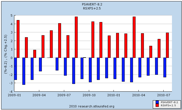
The tradeoff between savings and consumer spending is evident in the below graph. Since unfortunately the St. Louis FRED won't allow me to graph the rate of monthly change in the savings rate, the below is the best I can do. In the graph, the savings rate, normed to zero at its highest rate, is shown in blue. The change in retail sales, normed to zero at its lowest change, is shown in red, beginning of 2009.


While not exact, the general "mirror image" is clear. When the savings rate decreases (the blue line goes down), the change in retail spending increases (the red line goes up). When savings increase, the change in spending decreases. Note in particular the big increase in the savings rate in April of this year that coincided with a sharp decrease in the rate of retail spending. That was Pavlovian fear kicking in.

In tht regard, even if it is only one month, that consumers were comfortable saving a little less and spending a little more in July is a good sign that their Pavlovian fear may have begun to abate.

Yesterday's Market


Yesterday, the IEF's gapped higher at the open (a), fell a bit to the EMAs (b) and then gently rose for the rest of the day (c). However, most of their gain came from the opening gap higher.


For the last few days, the SPYs have found support in the (a) area. Yesterday, prices also found support and resistance between Fibonacci lines (b).


Prices gapped lower at the open (a), but quickly rebounded higher, printing strong bars (b) on decent volume. After hitting Fibonacci levels they got trapped in the EMAs for most of the day (c). They tried a near close sell off on rising volume (d) but quickly rebounded (e), finding resistance at Fibonacci levels.


On the daily chart, prices are still in a downward sloping wedge, between lines (a) and (b). Prices are also in a pretty tight range for the last week (c) at the bottom of the wedge.

Yesterday, oil prices took a big tumble, consolidating in a triangle pattern at the beginning of trading (A) and then falling for most of the rest of the day, rising to consolidate losses and find resistance at the EMAs several times (B and C). Prices eventually hit bottom at point (D).


Once again, oil prices are looking for support in the lower 70's area (A).


Wheat is still a correcting in a downward sloping pennant pattern (A). Notice that while momentum is decreasing (B), we're not seeing a price crash. The above chart pattern of a downward sloping consolidation pattern after a strong rally accompanied by decreasing momentum is pretty common.


Cattle has been in a strong rally (A) since the beginning of June. Prices are now approaching an important technical juncture as they decrease (C) gently to previous highs (B) and the upward sloping trend line (A).

Tuesday, August 31, 2010

A Break Down Of PCEs

What do we spend money on? To answer that question, let's take a look at personal consumption expenditures, or PCEs. These are the largest component of the GDP report. Click on all images for a larger image

First, note that PCE expenditures are broken down into services, non-durable and durable expenditures.
Services is the largest area of expenditures, accounting for 65% of PCEs. The three largest areas of service expenditures are housing, health care and "other".
After the "other" category in the non-durable category, we see that food, clothing and energy are the largest expenditures of the non-durable category.


And in the durable goods category, we see that recreational goods (think really big toys), cars and furnishings are the biggest components.


When we put all of this together, notice that housing and health care are the biggest areas of expense. Food and beverages for "off premises consumption" and financial services are also large areas of expense.

Bonddad In the NY Times

As some of you know, I also write a weekly column for 538.com. That site was recently purchased by the NY Times. My first blog entry as a New York Times Blogger is here.

Robert Barro - Paste Eater

Yesterday, Harvard economist Robert Barro penned an editorial that has to be one of the most insulting to intelligent economic researchers and should embarrass Harvard University for employing someone willing to put his personal ideology above the academic reputation of Harvard like Mr. Barro. This editorial espoused the idiotic notion that somehow had we only cut off unemployment benefits at 26 weeks instead of extending them (during the worst recession since the 30's) we would only be experiencing a 6.8% unemployment rate instead of the 9.5% rate we are currently at (not to discount U-6 which stands at 16.5%). Mr. Barro makes this claim not through actual intelligent research, but simply by using the long-term unemployment rate from the 1981 recession and applying that to our current situation as if they were identical (this is the kind of "research" one would expect from a high school student). By making this direct comparison Mr. Barro is either a) admitting that a Harvard economist has no idea about the differences between the recessions (which I will get into below) or b) that he is simply an intellectually dishonest shill. Which is it Mr. Barro?

To examine the actual data (which I might add is readily available to anyone with an internet connection these days, a fact perhaps Mr. Barro forgets), we can see that this recession is not at all like the 1981 recession and thus taking a direct comparison of long-term unemployment rates is simply wrong.

First, the 1981 recession was caused by the Federal Reserve hiking interest rates in an effort to combat the pervasive inflation of the times. As we can see from the graph below, the 1981 recession began with extremely high interest rates (I use the 10-year rate as a measure here to reflect not only the fed, but market expectations as well), while our current recession not only began with low rates (by historic standards, but also with a huge economic bubble (ie Housing) that did not exist prior to the 1981 recession).
treasurys
This graph also clearly highlights one of the prime movers of recovery from the 1981 recession, as a dramatic fall in interest rates at the end of the recession was a huge boon to the economy (and thus hiring).

Next, we should examine the savings rate. Back at the beginning of the 1981 recession, savings rates were high (allowing people and the economy to better sustain a job loss sans additional benefits) and when the recession ended, savings fell, again fueling a very sharp recovery.
savings81v07
While today, we can clearly see that the savings rate is on the rise (crimping current spending and current economic growth) and is still well below even the "recovery level" following the 1981 recession's end.

Drawing on Mr. Barro's argument that the 1981 recession = the 2007 recession, we should examine business loans, as these loans would typically indicate both demand/availability of credit to businesses that are looking to expand (or at least maintain current operations) and would have a direct impact on the ability of business to hire those people that would have jobs after 26 weeks had they simply not been lazy Americans.
loans81v07
Why, look at that, a quick examination of actual data shows that during the 1981 recession business loans stayed relatively flat (the uptick at the beginning was likely due to inflation), while during our "identical" recession they have fallen off a cliff. This indicates that businesses either a)do not have the access to credit to grow (ie hire) those lazy unemployed people or b) do not see the demand in the economy for growth (or both). Once again, data seems to indicate that Harvard made a poor decision in hiring Mr. Barro to teach (or "research") economics.

Finally, we can examine the JOLTS (Job Openings and Labor Turnover) data. This is a relatively new data source (it wasn't around during the 1981 recession) and perhaps because it is so new Mr. Barro didn't realize he could look here to back up his assertions. What we can see from JOLTS is that both job openings (private) and job hires (private) are still far below even the bottom levels from the last recession. Which is interesting, because according to Mr. Barro's theory, what we should be seeing are lots of job openings that go unfilled simply because those lazy unemployed don't want to work.
joltsopenings
Openings.
joltshiresprivate
Hires.
JOLTS also conveniently examines "quits" (ie people who quit their jobs), which we would expect to be much higher during a period of fantastic unemployment benefits (since you can qualify for UI benefits if you quit because hours were drastically reduced and/or pay was significantly cut), but when we examine the data we see that in fact quits are at a series low:
joltsquitrate
Once again displaying Mr. Barro's complete lack of even giving the data a cursory look before shooting his mouth (or in this case pen) off.

I think what we can conclude from all this is not necessarily that an extension of unemployment benefits has no impact at all on unemployment rates (but probably less so during such a deep recession like we are now mired in), but simply that Mr. Barro has shown himself to be the champion of the paste eaters and a person completely lacking in professional integrity as an economist.

Yesterday's Market


The SPYs were in a downward sloping channel yesterday, bounded by trend lines (a) and (b). Prices continually made lower lows and lower highs(c and d), eventually falling below the lower trend line at the close of trading on increased volume (e).


On the daily chart, prices are in a downward sloping channel (a and b) and are currently in a fairly tight trading range (c).


In the Treasury market, prices for the IEF gapped higher at the open (a) and started to use the 10 minute EMA and line (b) for technical support. Also note several downward sloping consolidation pennants (c) during the morning rally. After the rally prices moved in a sideways pattern for the rest of the day (d).


Notice that prices for the IEF found technical support at the 61.8% Fibonacci level.


Gold is still rallying (A). Notice the EMAs are still very bullish -- the shorter EMAs are above the longer EMAs and all the EMAs are moving higher. However, the last two days have printed incredibly weak candles (A) and the MACD is narrowing (D). Prices are also approaching important resistance levels (E).


The dollar was in a strong downtrend (A), until breaking out a few weeks ago (B). Prices have rallied, but have curved, moving into more of a holding pattern (C). Along the way, prices have consolidated in downward sloping pennant patterns (D). Yesterday, prices moved higher (E). Also notice the MACD is moving higher, although, like gold, the area between the indicator and signal line is decreasing (F).


Yesterday, the dollar was in a clear curving uptrend (A) that consolidated in downward sloping pennant patterns throughout the day (B).

Monday, August 30, 2010

State Tax Revenue Increasing


From the WSJ:

Overall tax revenue increased 2.2% in 47 states that have reported their receipts for the three months ended June 30, compared with the same period a year ago, according to a report to be released Monday by the Nelson A. Rockefeller Institute of Government at the State University of New York.

This marks the second quarter in a row of recovering tax collections—and follows five quarters of declines in revenue that hammered local-government budgets. The latest figures are still a mixed bag: Some states continue to see declining revenue, but those were offset by states that saw increases.

States continue to face financial pressure, in part because tax collections remain below the levels of two years ago. In addition, aid to state income provided by federal stimulus funds is starting to fall away. Signs that the economy is flagging add to the gloomy outlook for state coffers.

"Most states still show a mismatch between revenue and spending trend lines," said Robert B. Ward, deputy director of the Rockefeller Institute. "It's not time to put away the red ink yet."

Here's the accompanying graphic:


While the quarter to quarter increases are still small, they are there, indicating we are seeing an increase in activity.


Chip Sales Rise in July

From the WSJ:

Global chip sales rose 1.2% in July from a month earlier despite signs of a slowing economy, with results remaining sharply above prior-year levels, according to the Semiconductor Industry Association.

Chip sales in July reached $25.24 billion, up 37% on a yearly basis. The year-to-date increase was 47% above the moribund levels seen for the same period last year as by midyear the sector was starting to come out of a sharp slump in the wake of the financial crisis.

Meanwhile, "worldwide sales of semiconductors were strong in July despite growing indications of slower growth in the overall economy," said Brian C. Toohey, SIA's new president, who took the helm last month. Although a number of major manufacturers have emphasized limited visibility for the near-term, Mr. Toohey said the industry group continues to expect that sales growth this year will be in line with its prior forecast.

.....

However signs are emerging that the growth could stall amid a choppy economic recovery. Most recently, Intel Corp. on Friday cut its third-quarter revenue and margin outlook on weaker-than-expected consumer demand for PCs in developed markets.


Equipment and software expenditures have been partly responsible for GDP gains over the last four quarters. We'll see if that continues.

Credit Card Losses Are Slowing

From the FT:

US credit-card losses are falling faster than expected, with the six largest card issuers expected to earn nearly $10bn more in the coming 12 months than predicted, says a study by Moody’s.

Historically, US credit-card write-offs have tracked the unemployment rate. But for the first time in a decade, loans considered uncollectible by lenders are falling faster than the jobless rate, prompting analysts to revise earnings models.

The divergence from past experience reflects bank efforts to weed out risky borrowers, moves by consumers to pare back debts after the excesses of the past decade and new credit card rules intended to discourage reckless lending.

“We are getting back to an old-fashioned basis of lending, providing credit only to people who have the ability to repay,” said Curt Beaudouin, an analyst at Moody’s.

The agency expects the six leading credit card issuers to earn nearly $10bn more in pre-tax profits in the 12 months from July than it forecast in March: $2.7bn for Citigroup; $2.6bn for JPMorgan Chase; $2.5bn for Bank of America; $931m for Capital One; $552m for American Express and $658m for Discover.

This ties in with a drop in household debt and a lower financial obligation ratio. Consider these charts from the St. Louis Fed:


These developments have occurred at the same time as we've seen an increase in the savings rate.


In short, households are paying down their debt right now.


Yesterday's Market


Prices dropped after gapping at the open (a) but rebounded pretty quickly (b). After rallying, prices fell back to key support levels (c) before again moving higher. Notice that prices used the 10 minute EMA as technical support. Finally, prices ended near highs for the day.


On the IEF, notice that prices were in a tight range for a 6 days (a). In addition, prices had three major drops last week (b, c and d). In short, prices couldn't hold onto gains.


On Friday, the IEFs opened with a gap at the open and rallied into the 10 minute EMA before making a strong downward move (c). Notice that prices rallied into the EMAs, but found resistance at those levels on a regular basis.


While the 7-10 year Treasury ETF is still in an uptrend (a) it dropped hard on Friday (b).

After consolidating (A), copper broke out on Friday (B). Note the MACD is close to giving a buy signal (C).


Oil has been an underperforming commodity for the last 4-6 months according to Stockcharts, PERF charts. Recently, prices hit key support areas (A) and bounced higher (D). However, the shorter EMAs are below the longer EMAs, but the MACD may be close to a buy signal (C).